12 Easy Steps to speed up in Excel

1. Quickly add new data to the diagram

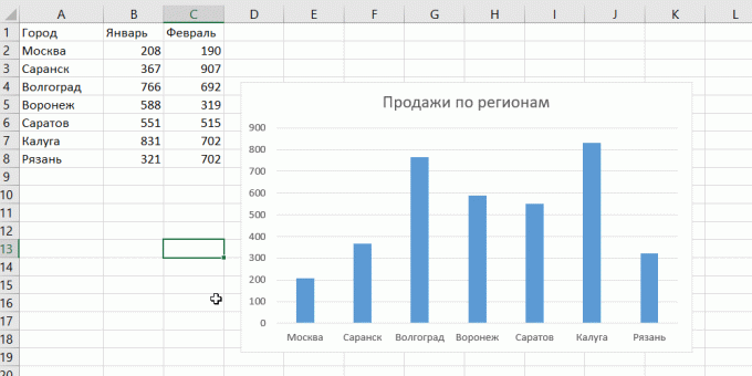
If charting on a sheet of new data to be added, you can simply select a range with the new information, copy it (Ctrl + C) and then paste directly into the diagram (Ctrl + V).

2. Instant filling (Flash Fill)

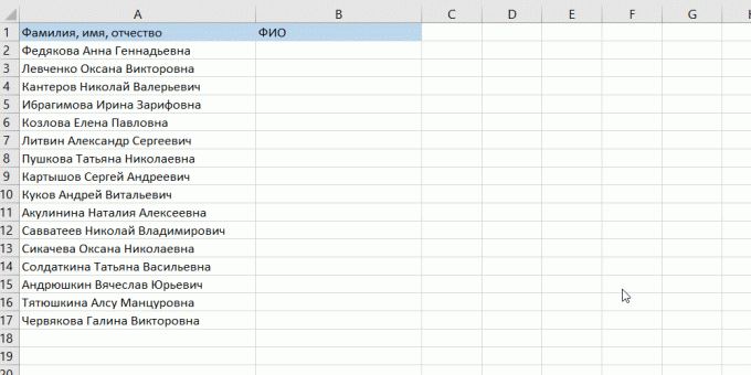
Suppose you have a list full name (Ivan Ivanov) that you will need to turn in a shortened (Ivanov I. AND.). To do this, you just need to start writing the desired text in the adjacent column by hand. On the second or third line, Excel will try to predict our actions and perform further processing automatically. Will only have to press the Enter key to confirm, and all the names will be converted instantly. Likewise, you can retrieve the names of the email, glue the name of the fragments, and so on.

3. Copying without violating formats

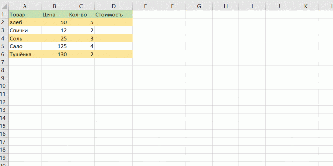
You probably know about a magic marker autocomplete. This slim black cross in the bottom right corner of the cell by pulling on which you can copy the contents of a cell or a formula to several cells. However, there is one unpleasant nuance is often breaks up the design table, as not only copied the formula, but the format of the cell. This can be avoided. Immediately after being pulled over a black cross, click on the smart tag - a special icon that appears in the lower right corner of the copied region.

If you select "Copy only values» (Fill Without Formatting), then Excel will copy your formula without format and will not spoil the appearance.

4. Displaying data from an Excel spreadsheet on the map

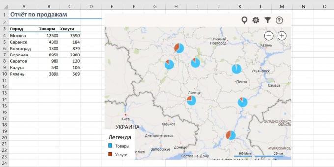
In Excel, you can quickly display the interactive map on your location, such as the sale of the cities. To do this, go to the "app store» (Office Store) on the tab "Insert» (Insert) and set out the plugin "Maps Bing» (Bing Maps). This can be done by direct link from the site by clicking on Get It Now.

After adding the module can select it from the drop down list of "My Android Apps» (My Apps) on the tab "Insert» (Insert) and place it on your worksheet. Remain set aside your cell data and click on Show Locations button in the card module, to see our data on it. If desired, the plug-in settings to select the type of color chart and to display.

5. Quick jump to the required sheet

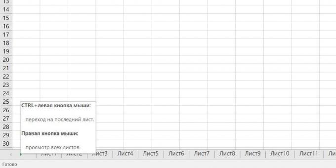
If the file number of worksheets exceeded 10, then guided them becomes difficult. Right-click on any of the buttons to scroll through the sheet tabs at the bottom left corner of the screen. You will see the table of contents, and on any desired sheet can be instantly jump.

6. Conversion rows into columns and vice versa

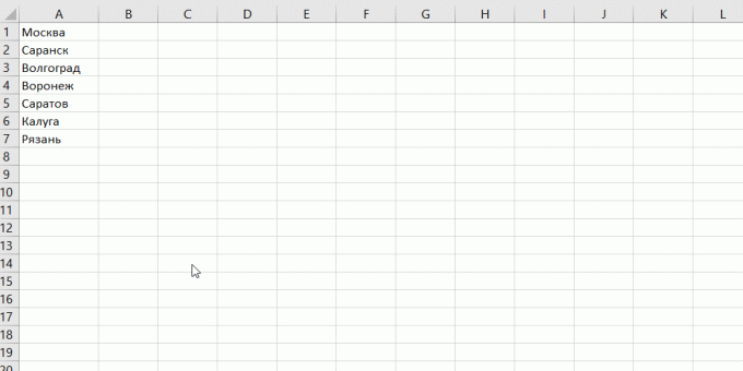
If you ever have to move your hands from the cell lines in the columns, then you'll appreciate the following trick:

1. Select the range.
2. Copy it (Ctrl + C) or by clicking the right mouse button, select "Copy» (Copy).
3. Right-click on the cell where you want to paste the data, and select from the following Paste Special from the context menu - the icon "Transpose» (Transpose). In older versions of Excel, there is no such icon, but you can solve the problem by using a special paste (Ctrl + Alt + V) and select "Transpose» (Transpose).

7. The drop-down list box

If any cell is assumed administered strictly defined set of values ​​of the allowed (e.g., 'yes' and "no" or only from the company's list of departments and so on), it can be easily arranged by using the drop-down list.

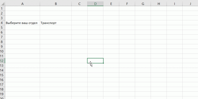
1. Select the cell (or a range of cells), which should be a limitation.
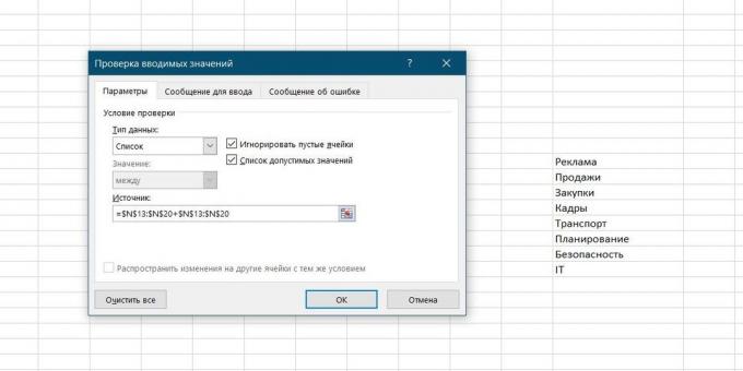
2. Click the "Data Validation" tab "Data» (Data → Validation).
3. In the dropdown list "type» (Allow), select "List» (List).
4. In the "Source» (Source) specify a range containing the reference embodiments of elements, which will subsequently fall on input.

8. smart table

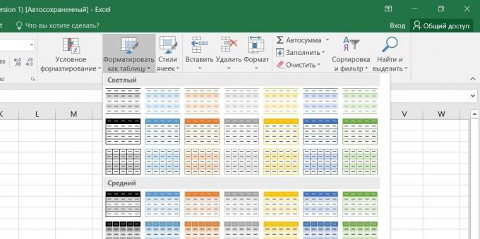
If you select a range of data and on the tab "Home" click on "Format as Table» (Home → Format as Table), then our list will be converted to smart table, which can many useful things:

1. Automatically expands as it append new rows or columns.
2. The entered formula will be copied automatically to the entire column.
3. Cap of this table is automatically assigned when you scroll, and it includes a filter button for selecting and sorting.
4. Appeared on the tab "Designer» (Design) in the following table, you can add the results of a string with automatic calculation.

9. Sparklines

Sparklines - is drawn directly into miniature cells chart clearly displays the dynamics of our data. To create them, click "Schedule» (Line) or "Histogram» (Columns) in the group "Sparklines» (Sparklines) tab "Insert» (Insert). In the window that opens, specify the range with the original numerical data and the cell where you want to display sparklines.

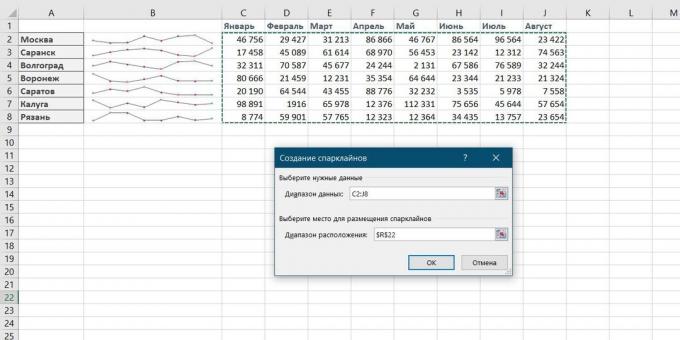
After clicking "OK» Microsoft Excel will create them in these cells. Appeared on the tab "Designer» (Design) you can further customize their color, style, enable the display of minimum and maximum values, and so on.

10. Recovering unsaved files

Imagine: you close the report, which were busy the last half of the day, and in the dialog box "Save changes to the file?" Suddenly for some reason presses "No". Office announces your heart-rending cry, but it was too late: the last few hours of work went down the drain.

In fact, there is a chance to rectify the situation. If you have Excel 2010, click on the "File» → «last» (File → Recent) and look in the lower right corner of the screen click the "Restore unsaved books» (Recover Unsaved Workbooks).

In Excel 2013 a slightly different path: "File» → «information» → «Versioning» → «Recover unsaved books» (File - Properties - Recover Unsaved Workbooks).

In later versions of Excel should open the "File» → «information» → «Book Management".

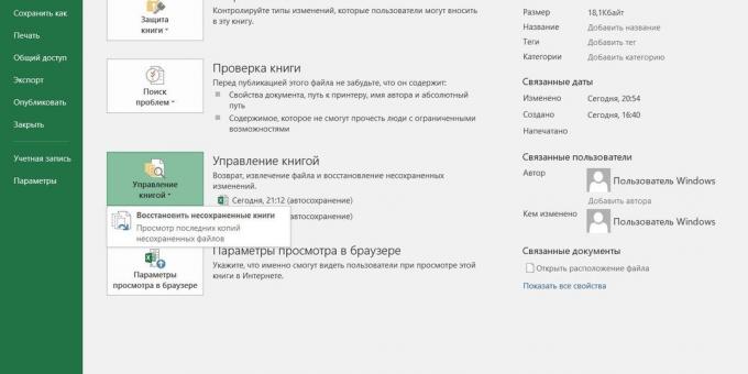
Open a special folder from Microsoft Office subsoil, where this is the case retained temporary copies of all created or modified but unsaved books.

11. Comparison of the two bands on the differences and similarities

Sometimes when working in Excel it is necessary to compare two lists and to quickly find items that are the same or different. That's the fastest and most intuitive way to do it:

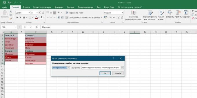
1. Select both of compared column (while Ctrl key).
2. Select the tab "Home» → «Conditional Formatting» → «Rules isolation cells» → «Duplicate values» (Home → Conditional formatting → Highlight Cell Rules → Duplicate Values).
3. Select "Unique» (Unique) in the drop-down list.

12. Selection (adjustment) calculation results under the desired values

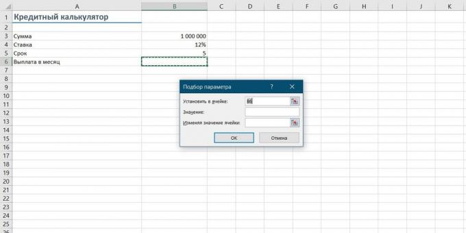
Have you ever picked up the input values ​​in your Excel calculation to get the desired result at the output? In those moments you feel hardened artilleryman: just a couple of dozen iterations "undershoot - flight" - and here it is, the long-awaited hit!

Microsoft Excel will be able to make such a fit for you, with faster and more accurate. To do this, click on the "Data" tab button "analysis" what if "," and then click "Seek» (Insert → What If Analysis → Goal Seek). In the window that appears, set the cell where you want to pick up the desired value, the desired result and the input cell that needs to change. After clicking on "OK» Excel performs up to 100 "shots" to pick your desired result to the nearest 0,001.